
An operator signs off a Class B+ design, the optical budget looks comfortable on the spreadsheet, and then the first 1:128 splitter is installed and every ONT sits within a decibel of its receiver sensitivity. The split ratio was picked from a marketing table rather than from the budget, and nothing downstream of the OLT can put that decibel back. The opposite mistake costs money just as quietly: paying for C+ optics across a network a 1:32 split would have served on standard B+ ports. Aligning split ratio, ODN class and reach is the cheapest engineering decision in an FTTH build, and it has to be made before a single splitter is ordered.
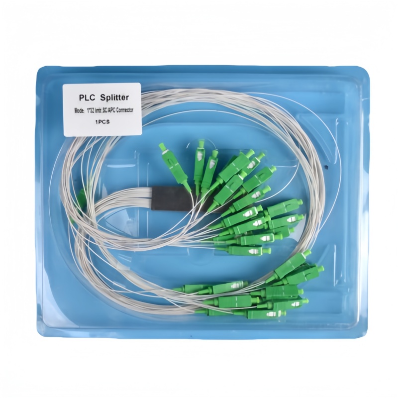
Why the Split Ratio Sets the Whole Bill of Materials
A PON optical budget is the difference between the launch power of an OLT port and the receiver sensitivity of the ONT, and the ITU-T class fixes how much of that difference the outside plant is allowed to consume. GPON defines its classes in ITU-T G.984.2; the 10G generations use the N and E classes in ITU-T G.987.2 and in the G.9807.1 series. The class is the envelope every splitter, closure, connector and fiber has to fit inside.
The split ratio matters because a passive splitter converts subscriber ports into decibels. Every doubling of port count costs roughly 3.0 dB of ideal splitting loss before the excess loss of the device itself, so the decision cascades: the ratio sets the ODN loss floor, the loss floor sets the required class, the class sets the OLT optics, and the optics set the price per port. Buyers who treat the ratio as a planning detail usually discover it as a cost line later.
| System | Class | Max ODN loss | Typical split ratio | Where it fits |
|---|---|---|---|---|
| GPON (ITU-T G.984.2) | B+ | 28 dB | 1:32 to 1:64 | Standard FTTH, 20 km class ODN |
| GPON (ITU-T G.984.2) | C+ | 32 dB | 1:64 to 1:128 | Long feeder or heavy splitting |
| XG-PON / XGS-PON (ITU-T G.987.2) | N1 | 29 dB | 1:32 to 1:64 | 10G upgrade reusing a B+ ODN |
| XG-PON / XGS-PON | N2 | 31 dB | 1:64 | Upgrade with marginal existing feeder |
| XG-PON / XGS-PON | E1 | 33 dB | 1:64 to 1:128 | Extended reach greenfield |
| XG-PON / XGS-PON | E2 | 35 dB | 1:128 | Rural and long-feeder routes |
Two details get missed when reading these classes. First, each class also has a minimum loss, so a link that measures too clean can overload the receiver just as a lossy link underruns it. Second, where GPON and XGS-PON share one ODN, the coexistence filter at the OLT adds roughly 0.5 to 1.0 dB that belongs in the budget, not in the margin.
What Each Split Ratio Costs in the ODN
Planar lightwave circuit splitters have well-behaved loss curves, which makes them easy to budget. The figures below are values to design against, not best-case numbers.
| Split ratio | Typical insertion loss | Max insertion loss | Uniformity (max) | Practical note |
|---|---|---|---|---|
| 1:2 | 3.4 dB | 3.8 dB | 0.4 dB | Commonly used at the OLT for port splitting |
| 1:4 | 7.1 dB | 7.4 dB | 0.5 dB | First stage of a cascaded design |
| 1:8 | 10.4 dB | 10.7 dB | 0.6 dB | Upper limit for FBT equivalents |
| 1:16 | 13.4 dB | 13.7 dB | 0.8 dB | Common MDU second stage |
| 1:32 | 16.8 dB | 17.1 dB | 1.0 dB | Comfortable on Class B+ |
| 1:64 | 20.5 dB | 21.2 dB | 1.5 dB | Requires Class C+ or better with real feeder length |
| 1:128 | 24.0 dB | 24.8 dB | 2.0 dB | Only with N2/E1/E2 class optics on short drops |
The step from 1:64 to 1:128 costs about 3.5 dB of measured loss. At 0.30 dB per kilometre at 1490 nm, that is the equivalent of roughly 11 km of feeder fiber given away to double the port count. Whether that trade is worth taking depends on where subscribers actually are, which is why the split decision belongs with the route survey, not at the end of procurement. Device technology matters too: a PLC versus FBT splitter comparison explains why PLC modules dominate above 1:8, and fiber optic splitter orders should be specified by ratio, polish and port count.

Worked Example: Class C+ at 1:64 and 1:128
Fixed overhead makes the arithmetic concrete. Take a mid-size ODN: a coexistence filter at the OLT, two mated connector pairs in the central office, six fusion splices across feeder and distribution, two mated pairs at the distribution point and the ONT, and a 3.0 dB allowance for ageing and temperature drift. That non-splitter overhead totals about 5.8 dB.
| Split ratio | Splitter loss (typical) | Total design loss | Spare inside Class C+ (32 dB) | Fiber reach at 0.30 dB/km |
|---|---|---|---|---|
| 1:16 | 13.4 dB | 19.2 dB | 12.8 dB | Protocol-limited, not budget-limited |
| 1:32 | 16.8 dB | 22.6 dB | 9.4 dB | Protocol-limited, not budget-limited |
| 1:64 | 20.5 dB | 26.3 dB | 5.7 dB | About 19 km of feeder and distribution |
| 1:128 | 24.0 dB | 29.8 dB | 2.2 dB | About 7 km, short-drop areas only |
The table explains why 1:64 on Class C+ is the default in most dense FTTH designs and why 1:128 is a niche choice at this class. Swapping typical splitter loss for maximum rated loss removes another 0.7 dB, which is 2 km of glass. If a project genuinely needs 1:128 at 15 km, the answer is not a better splitter; it is E1 or E2 optics with higher launch power, plus a platform check that the OLT supports that class on every port you intend to sell.
Cascaded Splitting: Cheaper Feeder, Dearer Decibels
A two-stage design of 1:4 followed by 1:16 looks arithmetically free: 7.1 dB plus 13.4 dB equals the 20.5 dB of a single 1:64 device. The loss is not the difference; the housing and connections around the second stage are.
A cascaded network needs at least one extra mated connector pair at the input of the second stage, typically 0.3 dB, and often a patched-through distribution panel. Practical penalty: 0.9 to 1.5 dB of extra loss compared with a single-stage splitter. What you buy for those decibels is granularity. A 1:4 feeder splitter stays in place while 1:16 modules are added only as subscribers connect, so the initial outlay matches the take-up rate, and spare ports can be reserved in a sealed fiber termination box rather than terminated and left dark. Brownfield builds that reuse an existing 1:4 feeder stage usually have no realistic alternative.
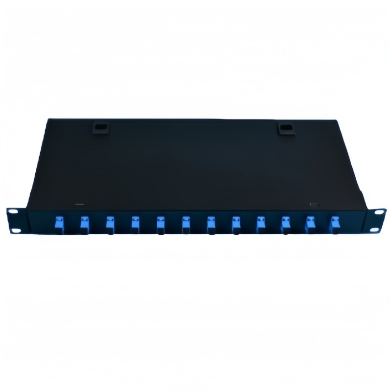
Components That Protect the Margin
Once the ratio and class are fixed, the remaining variable is component quality at every mated interface. Standard allowances are stable: a mated connector pair at 0.3 dB typical and 0.5 dB allowed, a fusion splice at 0.1 dB, and a mechanical splice at up to 0.3 dB. The FOA loss budget reference and the Fluke Networks fiber optic loss budget guide both work from those numbers, while TIA-568 sets the cabling framework the purchase specification should quote for structured cabling inside buildings.
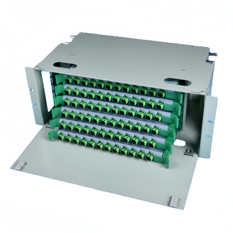
Polish discipline separates a working PON from a marginal one. PON ODNs are specified around angled physical contact connectors, and the central office is where the wrong cord does the most damage: a UPC patch cord mated into an APC adapter produces a reflection problem that shows up as unstable registration rather than as a clean loss number, and on the upstream 1310 nm band it can cost far more than the 0.5 dB allowance. Keep the polish consistent at every interface, use the ODF fiber optic distribution frame to terminate feeder without field splices, and buy tray-ready 12-core fiber pigtails with the same polish as the adapters in the closure.
Acceptance Plan for a Split ODN
A split PON cannot be validated with a single end-to-end test, because a splitter hides everything behind it from a one-ended measurement. Each stage needs its own record.
- Design sheet first: record the calculated loss per PON port for each split ratio, with splitter, connector and splice allowances plus margin, and make it the acceptance benchmark rather than the equipment datasheet.
- OTDR the feeder before splitters are loaded: at 1550 nm, with bidirectional traces, so the feeder and any mid-span splices have a recorded signature before downstream branches obscure the trace.
- Loss-test every drop with a light source and power meter: 1490 nm downstream and 1310 nm upstream, then compare against the class budget with at least 3 dB spare for ageing and dirty connectors.
- Check splitter uniformity per port: a 1:64 PLC module should hold within about 1.5 dB across ports; a wider spread points to a damaged port or a contaminated end face rather than a fiber fault.
- Confirm polish compatibility at every mated pair: a mismatched UPC and APC connection can pass a loss test and still fail on reflection, so inspect rather than assume.
- Deliver a per-port loss sheet with splitter serials and the OLT class: the next upgrade, whether XGS-PON coexistence or a move from 1:64 to 1:128, can then be planned on measured data.
Send Fenxi your PON port count, planned split ratios and target reach, and we will return a budget-checked bill of materials covering PLC splitters, terminal boxes, ODF units and matching pigtails and patch cords, with the loss each item contributes to the ODN written next to it.